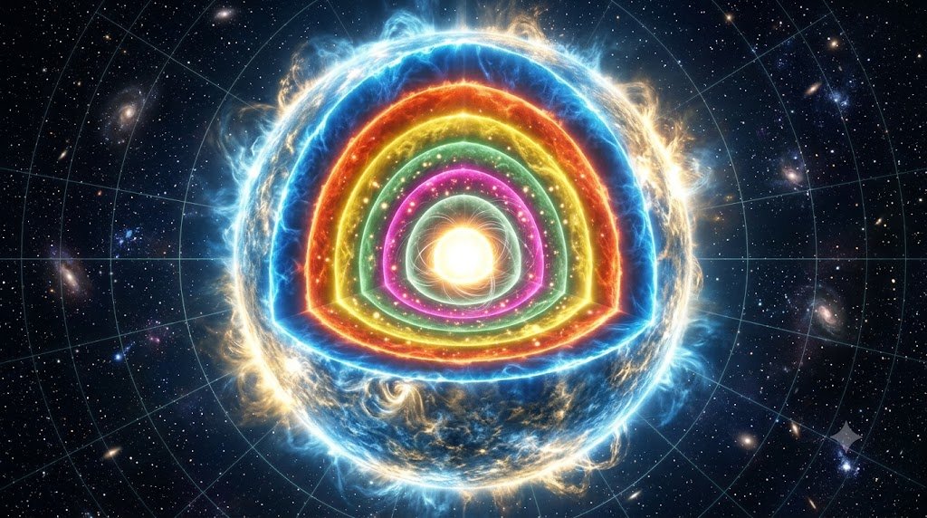
When we gaze into the nocturnal sky, stars appear as monochromatic pinpricks of light scattered across the velvety dark. Yet when that starlight is captured by an astronomical spectrograph and dispersed across its component wavelengths, it transforms into an intricate barcode of dark absorption lines and radiant emission bands. Spectroscopy is the foundational analytical technique of modern astrophysics. By analyzing stellar spectra, astronomers determine the surface temperature, chemical composition, surface gravity, rotational velocity, magnetic field strength, radial velocity, and evolutionary age of objects trillions of kilometers distant without ever leaving Earth. This comprehensive guide explores the physics of stellar spectral classification, the Harvard OBAFGKM sequence, the Yerkes luminosity classes, and the pivotal diagnostic framework of the Hertzsprung-Russell (H-R) Diagram.
1. The Physics of Stellar Radiation: Blackbody Curves and Wien’s Law
A star’s photosphere radiates electromagnetic energy across a continuous distribution of wavelengths, behaving very nearly like an idealized thermodynamic blackbody. The continuous emission spectrum generated by hot, dense plasma within the stellar photosphere is governed by Planck’s Radiation Law, which describes the spectral radiance as a function of temperature and wavelength:
1. Wien’s Displacement Law: The wavelength of peak emission (λ_max) is inversely proportional to the star’s absolute surface effective temperature (T_eff):
λ_max = b / T_eff (where b ≈ 2.898 × 10^-3 m·K).
Blistering stars (30,000 K) peak in the ultraviolet, intermediate stars like the Sun (5,778 K) peak in the visible green-yellow spectrum, and cool stars (3,000 K) peak in the infrared.
2. Stefan-Boltzmann Law: The total radiant energy emitted per unit surface area per second is proportional to the fourth power of temperature:
F = σ · T_eff⁴ (where σ ≈ 5.6704 × 10^-8 W·m^-2·K^-4).
Consequently, total stellar luminosity scales with surface area and temperature: L = 4 π R² σ T_eff⁴.
2. Atomic Absorption Physics: The Formation of Fraunhofer Lines
As continuous blackbody radiation travels outward from the dense, hot interior of the star, it passes through the cooler, less dense outer layers of the stellar atmosphere. Atoms and ions within these upper layers absorb specific discrete frequencies of photons that correspond exactly to the quantum energy differences between their electronic orbitals (ΔE = hν = hc/λ). When these excited electrons subsequently decay back to lower energy levels, they re-emit photons isotropically in all directions, creating prominent dark absorption gaps known historically as Fraunhofer Lines.
The Saha Ionization Equation and the Boltzmann Population Law
In the early twentieth century, astronomers initially assumed that differences in absorption line strengths among stars directly reflected differences in their chemical composition. If a star exhibited faint hydrogen lines, it was assumed to possess little hydrogen. This misconception was completely dismantled by astrophysicist Cecilia Payne-Gaposchkin in her groundbreaking 1925 doctoral dissertation.
Payne demonstrated that stellar atmospheres across the cosmos share a remarkably uniform chemical composition (overwhelmingly hydrogen and helium). The observed variations in spectral line strengths are almost entirely a thermodynamic consequence of temperature and ionization states, governed by two fundamental physical equations:
- Boltzmann Distribution: Determines the ratio of atomic populations occupying excited quantum states versus the ground state as a function of thermal kinetic energy: N_b / N_a = (g_b / g_a) · exp(-[E_b – E_a] / kT).
- Saha Ionization Equation: Quantifies the ionization equilibrium balance between neutral atoms and successive ionization stages based on temperature, electron density, and ionization potentials.
Hydrogen Balmer lines, for instance, originate exclusively from neutral hydrogen atoms whose single electron occupies the second energy level (n=2). In cool M-dwarf stars (3,000 K), virtually all electrons reside in the ground state (n=1), so optical Balmer absorption cannot occur. In blistering O-type stars (40,000 K), thermal energy is so violent that hydrogen atoms are stripped of their electrons entirely (ionized into bare protons), leaving no bound electrons to absorb light. Balmer lines reach their peak prominence exclusively at intermediate temperatures around 9,500 to 10,000 Kelvin—the exact surface temperature of A-type stars like Vega and Sirius.
3. The Harvard Spectral Sequence: O B A F G K M
Developed by Annie Jump Cannon, Williamina Fleming, and their colleagues at the Harvard College Observatory, the modern Morgan-Keenan (MK) Spectral Sequence arranges stars in order of decreasing effective photosphere temperature. The famous mnemonic “Oh Be A Fine Girl/Guy, Kiss Me” summarizes the sequence:
| Class | Effective Temp (K) | Photospheric Color | Dominant Spectral Features | Archetypal Example Stars |
|---|---|---|---|---|
| O | > 30,000 K | Deep Electric Blue | Ionized Helium (He II), weak neutral He, ionized C, N, O | Alnitak (Zeta Orionis), Mintaka |
| B | 10,000 – 30,000 K | Blue-White | Neutral Helium (He I) peak, rising Hydrogen Balmer lines | Rigel, Spica, Regulus |
| A | 7,500 – 10,000 K | Pure White | Maximum Hydrogen Balmer series, ionized metals (Fe II, Mg II) | Sirius, Vega, Altair, Deneb |
| F | 6,000 – 7,500 K | Yellow-White | Ionized Calcium (Ca II H & K lines), moderate Balmer lines | Procyon, Canopus, Polaris |
| G | 5,200 – 6,000 K | Yellow | Intense Ca II H & K, abundant neutral metals (Fe I), CH band | The Sun, Alpha Centauri A, Capella |
| K | 3,700 – 5,200 K | Orange | Strong neutral metal lines, emerging molecular TiO bands | Arcturus, Aldebaran, Pollux |
| M | 2,400 – 3,700 K | Reddish-Orange | Prominent Titanium Oxide (TiO) absorption bands, neutral Fe | Betelgeuse, Antares, Proxima Centauri |
Each major spectral letter is subdivided into ten decimal subclasses ranging from 0 (hottest) to 9 (coolest). For example, our Sun is classified precisely as a G2 star, indicating a surface temperature of 5,778 Kelvin, noticeably hotter than a G8 dwarf but cooler than a G0 star.
4. The Yerkes (M-K) Luminosity Classes: Pressure Broadening
Spectral class alone reveals a star’s surface temperature, but it does not specify whether the star is an ordinary dwarf or a bloated supergiant. To resolve this ambiguity, William Wilson Morgan, Philip C. Keenan, and Edith Kellman developed the Yerkes Luminosity Classification.
The physical mechanism behind luminosity classification is collisional pressure broadening (Stark Effect). In compact dwarf stars with high surface gravities (g = GM/R²), atmospheric gas pressure is extreme. The dense electric fields of adjacent ions perturb atomic energy levels, broadening spectral absorption lines into wide, shallow wings. In swollen, diffuse supergiants possessing immense radii and razor-thin atmospheric densities, atoms collide infrequently, producing razor-sharp, narrow spectral absorption lines.
• Class Ia-O / Ia+: Hypergiants or extremely luminous supergiants (e.g., VY Canis Majoris)
• Class Ia: Luminous Supergiants (e.g., Deneb, Rigel)
• Class Ib: Less luminous Supergiants (e.g., Betelgeuse, Polaris)
• Class II: Bright Giants (e.g., Mintaka)
• Class III: Normal Giants (e.g., Arcturus, Aldebaran)
• Class IV: Subgiants transitioning off the main sequence (e.g., Procyon)
• Class V: Main-Sequence Dwarf Stars fusing core hydrogen (e.g., The Sun – G2V)
• Class VI (sd): Subdwarfs (low metallicity halo stars)
• Class VII (D): Degenerate White Dwarfs (e.g., Sirius B – DA2)
5. Navigating the Hertzsprung-Russell (H-R) Diagram
Independently conceived by Ejnar Hertzsprung and Henry Norris Russell between 1910 and 1913, the Hertzsprung-Russell Diagram is the master map of observational astrophysics. By plotting stellar luminosity (or absolute magnitude) along the vertical y-axis against effective surface temperature (or spectral class / B-V color index) along the inverted horizontal x-axis, stars organize themselves into distinct, evolutionarily meaningful populations:
The Main Sequence: Stable Core Hydrogen Burning
Running diagonally from the top-left (hot, luminous O-stars) to the bottom-right (cool, dim M-dwarfs), the Main Sequence contains roughly 90% of all stars in the observable universe. Position along this band is dictated purely by mass. The interior of every main-sequence star is characterized by steady hydrostatic equilibrium powered by core hydrogen fusion.
The Giant and Supergiant Branches
Hovering in the upper-right quadrant are the Red Giants (Luminosity Class III) and Red Supergiants (Class I). These stars have exhausted their core hydrogen fuel and expanded dramatically. Despite their relatively cool surface temperatures (3,000–4,500 K), their colossal surface areas (A = 4πR²) yield extraordinary total luminosities hundreds to hundreds of thousands of times greater than the Sun.
The White Dwarf Graveyard
Located in the lower-left quadrant sits the White Dwarf Cooling Track. These objects are extremely hot (10,000 to over 100,000 K), radiating blistering ultraviolet emission. However, because their physical radii are compressed to roughly the size of Earth, their miniscule surface area produces exceptionally faint total luminosities (typically 0.001 to 0.0001 L☉).
6. The Power of Spectroscopic Parallax and Globular Cluster Isochrones
The synergy between spectral classification and the H-R diagram unlocks one of the most powerful distance-measuring tools in astronomy: Spectroscopic Parallax. When a distant star is too far away for direct trigonometric parallax measurements (such as those pioneered by the Gaia space telescope), astronomers obtain its high-resolution spectrum. From line ratios and pressure broadening, they determine its exact spectral type and luminosity class (e.g., G2V). By reading the corresponding absolute magnitude M directly from the calibrated H-R diagram and measuring the star’s apparent magnitude m, the physical distance d in parsecs is calculated via the Distance Modulus Formula:
m – M = 5 · log₁₀(d) – 5 + A_v
Where (m – M) is the distance modulus and A_v is interstellar dust extinction. This formulation allows astronomers to gauge distances across thousands of light-years across our galaxy.
Furthermore, when astronomers plot the H-R diagram of an entire globular star cluster, where all stars formed simultaneously from the same nebular cloud, they observe a sharp departure point along the main sequence known as the Main Sequence Turnoff Point. Because massive stars evolve faster, the turnoff point shifts progressively toward cooler, lower-mass stars as the cluster ages. By comparing the turnoff point with theoretical stellar evolutionary models (isochrones), astronomers accurately date the ages of globular clusters, providing a vital empirical lower limit on the age of the universe itself.
7. Modern Extensions: Brown Dwarfs and Unusual Spectral Types
In modern observational astrophysics, the classical Harvard sequence has been expanded to accommodate ultracool sub-stellar objects and peculiar stellar compositions. For objects whose masses fall below 0.075 to 0.08 M☉ (the hydrogen-burning minimum mass), core temperatures never reach the threshold required for sustained hydrogen fusion. These failed stars—known as Brown Dwarfs—are categorized under new spectral classes:
- L-Dwarfs (1,300 – 2,200 K): Deep infrared emitters dominated by metal hydrides (FeH, CrH) and clouds of liquid iron and silicate dust in their upper atmospheres.
- T-Dwarfs (700 – 1,300 K): Characterized by prominent methane (CH₄) and water vapor (H₂O) molecular absorption bands, resembling the atmospheres of giant gas planets.
- Y-Dwarfs (< 700 K): The coldest known sub-stellar objects, with room-temperature surface regimes dominated by ammonia (NH₃) absorption.
- Wolf-Rayet (WR) Stars: Massive, stripped-envelope stars undergoing catastrophic mass loss, showing broad, intense emission lines of helium, nitrogen (WN), and carbon (WC).
8. High-Resolution Spectroscopic Diagnostics: Zeeman Splitting and Rotational Broadening
Beyond determining basic temperature and surface gravity, modern high-resolution astronomical spectrographs extract profound physical details from line profiles. When a star rotates rapidly on its axis (such as Altair or Achernar, spinning at hundreds of kilometers per second), the approaching stellar limb blue-shifts absorption lines while the receding limb red-shifts them. This geometric integration across the visible stellar disk causes rotational line broadening, parameterized by v · sin(i), where i is the inclination of the stellar rotational axis relative to Earth’s line of sight.
Furthermore, magnetic fields on stellar surfaces split degenerate atomic energy levels through the Zeeman Effect. In the presence of a strong magnetic field, a single spectral line splits into a triplet or multiplet of polarized components. The wavelength separation between these components (Δλ_Z = (e / 4π m_e c²) · g_eff · λ² · B) scales directly with magnetic field strength B. Through Zeeman Doppler Imaging, astrophysicists reconstruct full two-dimensional surface maps of starspots, coronal loops, and complex magnetic topologies across distant solar analogs.
From classifying the blistering blue hypergiants in the Tarantula Nebula to cataloging the frigid brown dwarfs drifting silently through the solar neighborhood, spectral classification remains the supreme Rosetta Stone of the cosmos, allowing astronomers to read the life stories of stars written directly in light.