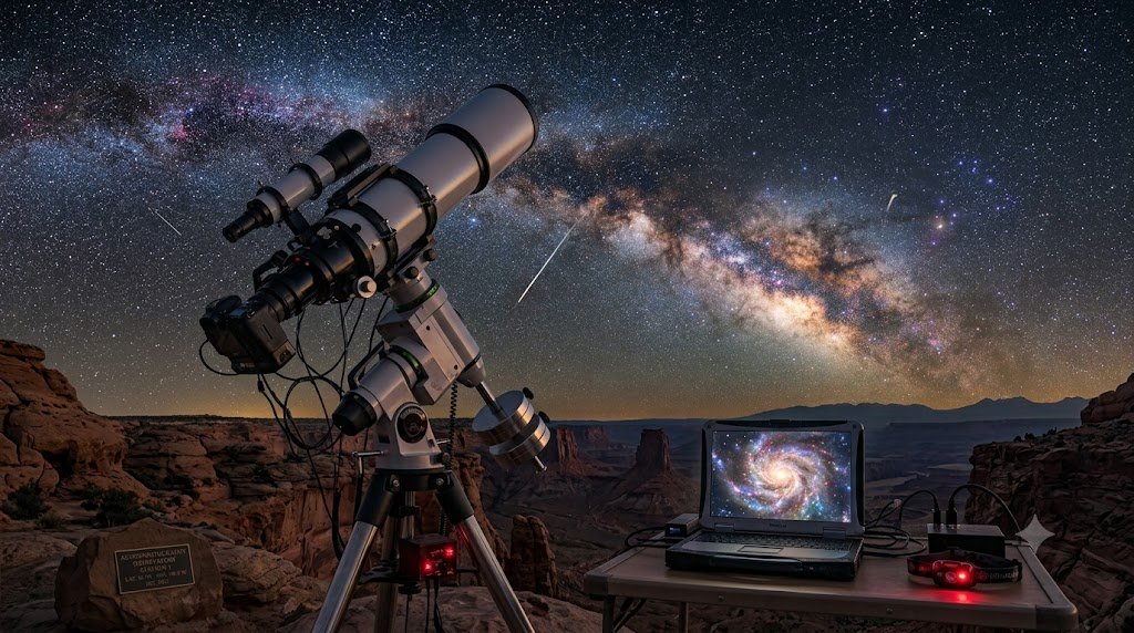
To gaze through a telescope eyepiece at a distant galaxy is an unforgettable visual experience, yet the human eye is constrained by its biological limitations: our retinas process light in real-time fractions of a second (roughly 1/10th of a second exposure time), rendering faint nebulae as soft, monochrome gray clouds. Deep-Sky Astrophotography liberates astronomy from biological limits. By utilizing silicon semiconductor sensors capable of accumulating incoming photons over minutes, hours, and days, astrophotography unveils the magnificent hidden colors of the universe: glowing red emissions of ionized hydrogen, electric turquoise filaments of doubly ionized oxygen, and intricate brown dust rifts stretching across cosmic space. Yet capturing crisp, pinpoint long-exposure astrophotographs is one of the most demanding technical disciplines in modern computing and physics. This comprehensive treatise explores the semiconductor physics of CMOS/CCD sensors, equatorial tracking mechanics, autoguiding loops, signal-to-noise ratio (SNR) mathematics, calibration frames (Darks, Flats, Biases), and the image stacking workflow.
1. Sensor Physics: Converting Photons into Digital Electrons
At the heart of every modern astronomical camera lies a silicon sensor—historically a Charge-Coupled Device (CCD), now predominantly a modern Complementary Metal-Oxide-Semiconductor (CMOS) sensor (such as Sony’s back-illuminated Exmor IMX series).
• The Photoelectric Effect: When an incoming photon strikes a silicon pixel, it excites an electron from the valence band into the conduction band, generating an electron-hole pair. The liberated photoelectron is captured within an electric potential well inside the pixel.
• Quantum Efficiency (QE): The percentage of incident photons that successfully liberate photoelectrons. While traditional film photography possessed a miserable QE of barely 2% to 3%, modern back-illuminated BSI-CMOS sensors achieve staggering Quantum Efficiencies of 80% to 91%, capturing virtually every photon focused onto their surface.
• Full Well Capacity & Dynamic Range: Full well capacity represents the maximum number of electrons a single pixel can hold before saturating (spilling over into adjacent pixels, or blooming). Large pixels (e.g., 5.76 μm) hold 50,000+ electrons, providing immense dynamic range between faint background nebulosity and brilliant stellar cores. Small pixels (e.g., 2.4 μm) offer high spatial sampling on short-focal-length scopes but saturate faster.
2. The Signal-to-Noise Ratio (SNR): The Ultimate Metric
The single most critical concept in astrophotography is the Signal-to-Noise Ratio (SNR). In astronomical imaging, individual exposures are not noisy because there is something wrong with the camera; they are noisy because nature itself is fundamentally probabilistic. Light arrives at the sensor according to Poisson statistics, exhibiting inherent Photon Shot Noise.
The total noise (σtotal) in an image is the quadrature sum of independent noise sources:
σtotal = √(Nsignal + Nsky_glow + Nthermal_dark + Nread2)
• Photon Shot Noise: Inherent statistical fluctuation equal to the square root of the incoming photon count: σshot = √N.
• Read Noise (Nread): Electronic noise generated by the on-chip analog-to-digital converter (ADC) during the readout process. Modern CMOS sensors feature ultra-low read noise (1.0 to 1.5 e−), enabling short sub-exposures.
• Thermal Dark Current: Spontaneous generation of thermal electrons within the silicon lattice without light, doubling roughly every 6°C increase in sensor temperature. Dedicated astrophotography cameras incorporate Thermoelectric Peltier Cooling (TEC), maintaining the sensor at -10°C to -20°C below ambient to virtually eliminate thermal noise.
The Power of Stacking: When you stack N separate exposures of identical duration, the desired celestial signal increases linearly with N, while random noise increases only with √N. Consequently, the Signal-to-Noise Ratio improves with the square root of the number of frames:
SNR ∝ √N
Stacking 16 frames doubles the SNR; stacking 64 frames quadruples it; stacking 100 frames yields a tenfold increase in image purity and clarity!
3. The Tracking Mount: Precision Celestial Mechanics
Earth rotates on its axis at roughly 15 arcseconds per second. If an astrophotographer opens a camera shutter for just 5 seconds through a telescope without a tracking mount, stars streak into blurry lines. Capturing 5-minute exposures of faint galaxies requires a precision German Equatorial Mount (GEM) or Harmonic Strain-Wave Mount aligned precisely with Earth’s rotational axis.
Polar Alignment: The Foundation of Round Stars
The Right Ascension (RA) axis of an equatorial mount must be mechanically aligned parallel to Earth’s polar axis. Any misalignment between the mount’s RA axis and the celestial pole produces field rotation: stars in the center of the frame remain round, but stars in the corners streak into concentric circular arcs over long exposures. Modern electronic polar alignment tools (such as software plate-solving algorithms in ASIAIR, N.I.N.A., or SharpCap) achieve polar alignment accuracy under 30 arcseconds in less than three minutes.
Periodic Error and Sub-Arcsecond Autoguiding
Even the finest machined worm gears in equatorial mounts possess microscopic physical imperfections, causing the mount tracking speed to oscillate slightly fast and slow in a repeating cycle known as Periodic Error (PE).
To counteract periodic error, wind gusts, and mechanical flexure, astrophotographers employ an Autoguider. A small secondary guide scope (or an Off-Axis Guider prism in the primary light cone) coupled to a sensitive CMOS camera continuously monitors a single guide star at 1-second intervals. Software (such as Open-Source PHD2) calculates the centroid position of the guide star with sub-pixel precision. If the star drifts by even 0.2 arcseconds, PHD2 immediately sends corrective directional pulses via pulse-guiding to the mount motors, locking the telescope onto its target with sub-arcsecond tracking accuracy for indefinitely long exposures.
4. Calibration Frames: The Fourfold Mathematical Requirement
Raw astronomical exposures (called Light Frames) contain unwanted sensor artifacts: fixed thermal patterns, hot pixels, dust shadows, and optical vignetting. Raw lights cannot simply be averaged together; they must first undergo rigorous mathematical calibration using three distinct types of Calibration Frames:
| Frame Type | Optical Setup | Exposure Duration | Physical Purpose |
|---|---|---|---|
| Light Frames | Telescope focused on celestial target | Long exposure (e.g., 120s to 300s) | Captures desired astronomical photons from target + skyglow + sensor artifacts |
| Dark Frames | Lens cap securely on (zero light) | Identical duration, gain, and temp as Lights | Measures thermal dark current and fixed hot pixels; subtracted from Light and Flat frames |
| Flat Frames | Diffused, uniform white light source (tracing panel) | Short (historically until histogram hits 50%) | Maps optical vignetting (dark corners) and dust motes on sensor glass; divided into Light frames |
| Bias Frames (or Dark Flats) | Lens cap on (zero light) | Shortest possible shutter speed (e.g., 1/4000s) | Measures electronic readout noise baseline and fixed pattern noise of ADC; subtracted from Flats |
For every pixel in each light frame, the calibrated intensity (Ical) is calculated via:
Ical = (Light − Master_Dark) / (Master_Flat − Master_Bias) × Mean(Master_Flat)
This elegant mathematical normalization completely erases dust donut rings, corrects corner falloff vignetting, and extinguishes thousands of blazing white hot pixels, leaving behind a pristine, geometrically flat, calibrated dataset.
5. Color Strategies: One-Shot Color (OSC) vs. Mono Narrowband (SHO)
Astrophotographers divide into two broad camps based on optical filtering and camera architecture:
One-Shot Color (OSC) Cameras
OSC cameras utilize a Bayer Matrix of microscopic red, green, and blue dye filters arranged in a grid (typically RGGB) directly over the sensor pixels. A single exposure captures full color information, which software reconstructs through an interpolation algorithm called debayering. OSC cameras are convenient, fast, and ideal for broadband targets like galaxies and reflection nebulae, but they lose resolution because 75% of pixels reject light of non-matching colors.
Monochrome Cameras and Narrowband Imaging (The Hubble Palette)
Monochrome sensors have no Bayer matrix; 100% of their pixels collect all incoming photons with maximum spatial sharpness. To create color images, the photographer cycles a motorized filter wheel containing specialized optical filters in front of the sensor:
Narrowband filters feature ultra-narrow passbands (typically 3 nm to 7 nm wide) centered on the precise quantum emission lines of hot interstellar gases:
• Hydrogen-Alpha (Hα – 656.3 nm): Deep ruby red; the ubiquitous tracer of ionized hydrogen in star nurseries.
• Oxygen-III (O-III – 500.7 nm): Vivid teal/cyan; emitted by intensely energetic ionizing radiation from white dwarfs and O-type stars.
• Sulfur-II (S-II – 671.6 nm): Deep crimson; illuminates shock boundaries where stellar winds collide with cold molecular clouds.
The Hubble Palette (SHO): Because both Hα and S-II emit in nearly identical shades of deep red, NASA Hubble scientists created a false-color mapping to highlight distinct chemical structures:
• Sulfur-II → Red Channel
• Hydrogen-Alpha → Green Channel
• Oxygen-III → Blue Channel
This mapping transforms chaotic reddish clouds into the breathtaking golden, amber, and cyan pillars made world-famous by the Pillars of Creation in the Eagle Nebula. Furthermore, because narrowband filters reject 98% of light pollution, narrowband astrophotography can produce pristine, research-grade images directly from downtown metropolitan centers!
6. The Image Processing Pipeline: From Linear Data to Final Masterpiece
Once calibrated frames are aligned (registered) and stacked using specialized astrophotography software (such as PixInsight, Siril, or Astro Pixel Processor), the resulting master file is a 32-bit linear image that looks entirely black to the human eye. Transforming this linear data into a stunning final image follows a rigorous mathematical workflow:
| Processing Phase | Algorithm / Operation | Physical & Computational Goal |
|---|---|---|
| 1. Background Extraction | Dynamic Background Extraction (DBE / GraXpert) | Models and subtracts light-pollution gradients and lunar illumination across the frame |
| 2. Color Calibration | Spectrophotometric Color Calibration (SPCC) | Plate-solves the field, compares thousands of star colors against Gaia satellite photometric catalogs to establish true physical white balance |
| 3. Deconvolution & Denoising | Point Spread Function (PSF) deconvolution & AI Wavelets (RC-Astro BlurXTerminator / NoiseXTerminator) | Mathematically reverses atmospheric seeing blur and optical aberrations to restore diffraction-limited star profiles, while separating noise from genuine nebulosity |
| 4. Non-Linear Stretching | Generalized Hyperbolic Stretch (GHS) / MaskedStretch | Transitions data from 32-bit linear space to human-visible non-linear tones without blowing out bright stellar cores |
| 5. Star Removal & Tone Tuning | StarNet++ / StarXTerminator separation | Isolates stars onto a separate layer, allowing deep curves, local contrast boosts, and saturation enhancement on faint nebulosity without bloating stars |
7. Essential Equipment Configurations for Beginners and Advanced Imagers
To avoid common gear-purchasing mistakes, astrophotographers should invest in balanced systems matched to their technical experience:
• The Smart Telescope Revolution: (e.g., ZWO Seestar S50, DWARF II). Fully automated, all-in-one robotic units containing optics, camera, tracking mount, and internal stacking computer. Operated via smartphone app, they allow absolute beginners to capture colorful deep-sky images in minutes with zero manual setup.
• The Wide-Field Tracker Rig: A sturdy photographic tripod, motorized star tracker (e.g., Sky-Watcher Star Adventurer GTi), mirrorless/DSLR camera, and a fast telephoto lens (e.g., 135mm f/2 or 250mm f/4.9). Ideal for sweeping Milky Way panoramas, the Andromeda Galaxy, and massive emission regions like the North America Nebula.
• The Dedicated Deep-Sky Refractor Rig: A 70 mm to 80 mm APO triplet refractor, dedicated cooled CMOS camera (e.g., ZWO ASI533MC Pro), auto-guider scope, electronic automatic focuser (EAF), and computer controller (e.g., ZWO ASIAIR Plus or Mini-PC running N.I.N.A.) riding on a HEQ5-class equatorial mount. This setup delivers pinpoint stars, automated autofocusing, meridian flipping, and unattended multi-hour imaging all night long.
8. Total Exposure Integration Time: Revealing the Invisible Universe
In deep-sky astrophotography, the most profound transformative variable is total integration time. While a single five-minute exposure of the Andromeda Galaxy reveals its bright core and prominent dust lanes, accumulating ten to twenty hours of exposure time fundamentally changes the image depth.
• The 2-Hour Baseline: Eliminates primary read noise and background shot noise, delivering clean, sharp spiral arms and bright planetary nebulae suitable for digital sharing.
• The 5-to-10-Hour Threshold: Unlocks ultra-faint outer galactic halos, delicate tidal tails from ancient galactic mergers, and faint background galaxy swarms residing billions of light-years away.
• The 20+ Hour Ultra-Deep Field: Captures the ghostly, faint luminescence of the Integrated Flux Nebula (IFN)—whispy high-latitude cirrus dust clouds floating thousands of light-years above the plane of the Milky Way, illuminated only by the collective starlight of our entire galaxy.
Astrophotography is the sublime convergence of optics, quantum mechanics, computer vision, and artistic expression. Each captured sub-exposure is a frozen fragment of time: an enduring tribute to humanity’s capacity to reach across unfathomable cosmic distances and preserve the majestic beauty of the universe.