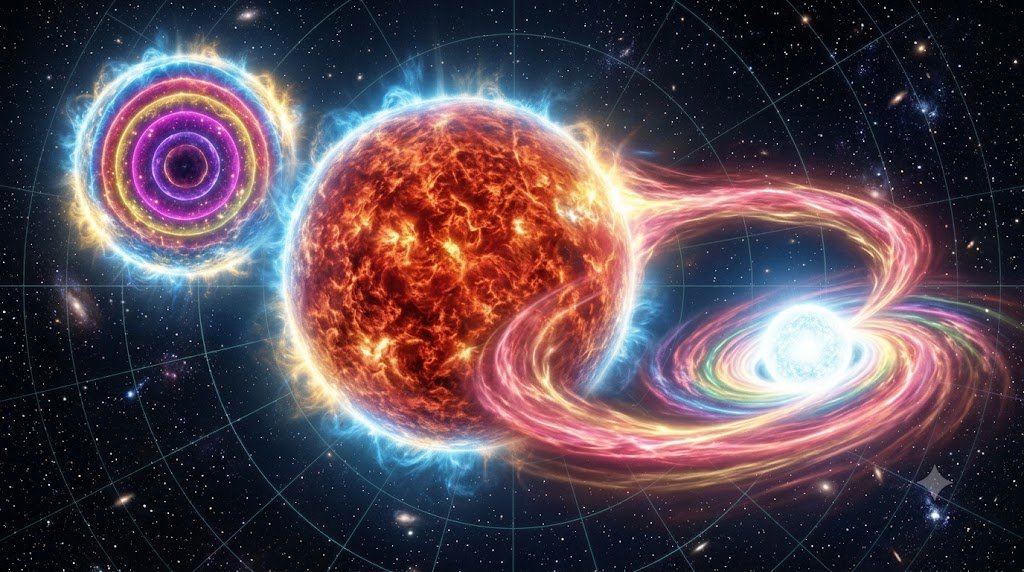
To the casual observer, the constellations appear as tranquil, unchanging monuments of eternity. Yet across cosmic timescales, and often over timescales of days or hours, the stellar heavens are alive with dynamic variability. Stars expand, contract, exchange gargantuan streams of plasma with orbital companions, and erupt in cataclysmic thermonuclear detonations that outshine entire galaxies. Variable stars and binary systems are not mere astronomical curiosities; they are precision astrophysical laboratories. They allow astronomers to measure fundamental stellar masses, chart the geometric expansion rate of the universe, and probe the most extreme physics of relativistic degenerate matter. This comprehensive guide explores pulsating variable stars, eclipsing and interacting binaries, and the explosive taxonomy of supernovae that define our cosmic distance ladder.
1. The Taxonomy of Stellar Variability: Intrinsic versus Extrinsic
Astronomers broadly classify variable stars into two primary physical categories:
1. Intrinsic Variables: Physical changes within the star itself induce luminosity variations. These include pulsating variables (e.g., Cepheids, RR Lyrae, Mira variables), eruptive variables (flare stars, luminous blue variables), and cataclysmic or explosive variables (novae, supernovae).
2. Extrinsic Variables: Luminosity fluctuations perceived by an observer are caused by geometric or orbital mechanisms rather than physical changes in the star’s intrinsic energy output. These include eclipsing binary systems and rotating spotted stars.
2. Pulsating Variables: The Kappa Mechanism and the Instability Strip
Pulsating variables periodically swell and shrink, causing their surface area, effective temperature, and luminosity to oscillate with mathematical regularity. On the Hertzsprung-Russell diagram, these stars occupy a nearly vertical swath known as the Instability Strip, which intersects the horizontal branch and extends through the supergiant domain.
The Valve Analogy: The Eddington Kappa Mechanism
Under normal stellar conditions, compressing a gas layer increases its temperature, which decreases its opacity (opacity scales inversely with temperature via Kramers’ opacity law: κ ∝ ρ · T^(-3.5)). As opacity drops, radiation escapes more easily, cooling the layer and allowing gravity to re-compress it. This negative feedback stabilizes ordinary stars.
However, within the Instability Strip, stars possess a sub-surface layer of partially ionized helium (the He II ionization zone). When this layer is compressed, the added thermal energy goes into ionizing helium (He⁺ → He²⁺ + e⁻) rather than raising kinetic temperature. The freed electrons drastically increase the local opacity via electron scattering: opacity rises upon compression. This layer acts as an internal heat valve, trapping outward radiant energy beneath it. The accumulated radiation pressure then forcefully pushes the outer atmospheric envelope outward.
As the star expands, the He II layer cools and recombines with free electrons, causing opacity to plummet. Trapped radiation escapes freely into space, pressure drops, and gravity pulls the outer envelope back inward, resetting the cycle. This cyclic pulsation engine is called the Kappa Mechanism (or Eddington Valve).
Classical Cepheids and the Leavitt Period-Luminosity Law
Among pulsating variables, Classical (Type I) Cepheids are the most renowned. In 1908, Harvard astronomer Henrietta Swan Leavitt analyzed Cepheid variables in the Small Magellanic Cloud. Because all stars within the cloud were situated at roughly the same physical distance from Earth, Leavitt made a historic discovery: a star’s apparent brightness was strictly correlated with its pulsation period. Longer period Cepheids were intrinsically far more luminous than shorter period Cepheids:
For Classical Cepheids, the mean absolute visual magnitude M_V is parameterized as:
M_V = -2.81 · log₁₀(P) – 1.43 (where P is the pulsation period in days).
By measuring a distant Cepheid’s light curve period with an optical telescope, astronomers immediately calculate its true intrinsic absolute magnitude M. Comparing this to its observed apparent magnitude m unlocks the exact distance to its host galaxy via the distance modulus. In 1923, Edwin Hubble famously used Cepheid V1 in the Andromeda “Nebula” (M31) to prove that Andromeda was an independent island galaxy millions of light-years away, expanding humanity’s known universe by billions of times.
RR Lyrae Variables: Galactic Halo Chronometers
Smaller and older than Cepheids, RR Lyrae variables are low-mass, horizontal-branch stars that pulsate with periods between 0.2 and 1.0 days. Remarkably, virtually all RR Lyrae stars possess nearly identical average absolute visual magnitudes around M_V ≈ +0.7, regardless of their period. Consequently, they serve as excellent “standard candles” for charting the distances and 3D geometric distribution of globular clusters and the Milky Way’s galactic halo.
3. Binary Star Systems: Orbital Mechanics and Stellar Mass Weighing
More than 50% of solar-type stars and upwards of 80% of massive O- and B-type stars do not drift in isolation; they are bound into gravitationally coupled binary or multiple star systems. Binary systems are the single most authoritative tool in astronomy for measuring fundamental stellar masses.
Visual, Astrometric, and Spectroscopic Binaries
Depending on orbital separation and distance from Earth, binary systems present different observational signatures:
- Visual Binaries: Both individual stellar components can be spatially resolved through optical telescopes (e.g., Albireo in Cygnus). Tracking their orbital motion over years allows direct determination of orbital semi-major axes and periods.
- Spectroscopic Binaries: The stars are too close together to resolve visually, but their orbital velocities induce alternating Doppler shifts in their spectral absorption lines. In double-lined spectroscopic binaries (SB2), absorption lines split and recombine periodically as one star approaches Earth while the other recedes.
- Eclipsing Binaries: The orbital plane of the pair is oriented edge-on toward Earth’s line of sight, causing the stars to periodically transit across and eclipse one another (e.g., Algol, the “Demon Star” in Perseus). High-precision photometric light curves reveal the stars’ exact physical radii, orbital inclinations, and surface temperature ratios.
By applying Newton’s gravitational formulation to binary orbital motions, the combined mass of both stars is determined directly:
M₁ + M₂ = (4 π² / G) · (a³ / P²)
Where a is the semi-major axis of the relative orbit and P is the orbital period. When combined with radial velocity ratios (M₁ / M₂ = v₂ / v₁), astronomers calculate the exact individual mass of each star.
4. Close Interacting Binaries: Roche Lobe Overflow and Accretion Dynamics
When two stars orbit in extreme proximity, their gravitational interaction enters the regime of the Roche Equipotential Model. The region of gravitational dominance surrounding each star is bounded by a teardrop-shaped boundary called the Roche Lobe. These two lobes touch at a gravitational saddle point known as the Inner Lagrangian Point (L1).
As the more massive primary star evolves off the main sequence and expands into a red giant, its physical radius can swell beyond its Roche lobe—a state known as Roche Lobe Overflow (RLOF). Matter from the giant’s outer convective envelope streams across the L1 point, spiraling toward the compact secondary companion. Because of angular momentum conservation, the infalling gas cannot plunge directly onto the companion’s surface; instead, it circularizes into a blazing, turbulent accretion disk governed by viscous magnetohydrodynamics.
Cataclysmic Variables, Classical Novae, and Dwarf Novae
If the mass-accreting companion is a carbon-oxygen white dwarf, the system is classified as a Cataclysmic Variable (CV). Hydrogen-rich gas pulled from the donor star accumulates onto the surface of the white dwarf, compressing into a dense, degenerate shell. As the base of this hydrogen layer reaches temperatures of 10 to 20 million Kelvin, electron degeneracy triggers a runaway thermonuclear explosion: a Classical Nova. The white dwarf blasts off its accumulated surface shell, brightening by up to 15 magnitudes (a factor of a million), but the underlying degenerate core survives intact to repeat the cycle over millennia.
5. Supernovae: The Great Cosmic Detonations
While classical novae are surface explosions that leave the white dwarf intact, Supernovae represent the complete, cataclysmic destruction of the progenitor star. Supernovae are categorized observationally by their spectral signatures and physically by their detonation engines:
| Supernova Type | Physical Mechanism | Defining Spectral Feature | Typical Peak Absolute Mag | Remnant Produced |
|---|---|---|---|---|
| Type Ia | Thermonuclear Disruption of White Dwarf at Chandrasekhar Limit | No Hydrogen; Prominent ionized Silicon (Si II at 615 nm) | M_V ≈ -19.3 (Uniform Standard Candle) | No central remnant (Complete disruption into Fe-group ash) |
| Type Ib | Core Collapse of Massive Star stripped of Hydrogen envelope | No Hydrogen; Prominent neutral Helium (He I at 588 nm) | M_V ≈ -17 to -18 | Neutron Star or Black Hole |
| Type Ic | Core Collapse of Massive Star stripped of both H and He | No Hydrogen; No Helium; Lines of O I, Ca II, Mg II | M_V ≈ -16 to -18 | Neutron Star, Black Hole, or Gamma-Ray Burst engine |
| Type II-P / II-L | Core Collapse of Massive Star retaining vast Hydrogen envelope | Strong Hydrogen Balmer absorption and P-Cygni emission | M_V ≈ -16.5 to -18.5 | Neutron Star (Pulsar) or Black Hole |
Type Ia Supernovae and the Accelerating Expansion of the Universe
Type Ia supernovae originate from carbon-oxygen white dwarfs that accrete mass from a binary companion or merge with another white dwarf. Because carbon ignition ignites under degenerate conditions at almost exactly the Chandrasekhar Mass (1.44 M☉), every Type Ia explosion releases a nearly identical quantity of kinetic energy and radioactive Nickel-56. Consequently, their peak luminosity is extraordinarily uniform, making them the premier “standard candles” for measuring cosmological distances across billions of light-years.
In 1998, two independent research collaborations—the High-Z Supernova Search Team and the Supernova Cosmology Project—used Type Ia supernovae to measure the cosmic expansion rate over cosmological time. To universal astonishment, distant Type Ia supernovae appeared noticeably fainter than predicted by a decelerating or matter-dominated universe. The data proved that the expansion of the universe is not slowing under gravity; it is actively accelerating, driven by a mysterious negative pressure dubbed Dark Energy (accounting for roughly 68% of the total energy density of the cosmos).
6. Supernova Remnants and Cosmic Ray Acceleration
The aftermath of a core-collapse or thermonuclear supernova expands into the interstellar medium at initial velocities exceeding 10,000 to 20,000 kilometers per second. The resulting Supernova Remnant (SNR)—such as the Crab Nebula (M1), Cassiopeia A, or the Cygnus Loop—sweeps up ambient interstellar gas in a massive shock front that glows brilliantly across radio, optical, X-ray, and gamma-ray wavelengths.
Within these turbulent shock fronts, charged particles (protons and atomic nuclei) scatter back and forth across magnetic inhomogeneities, gaining energy through Fermi Shock Acceleration. Supernova remnants are the primary cosmic accelerators that generate galactic Cosmic Rays—relativistic subatomic particles that travel near the speed of light, penetrating planetary atmospheres and fueling interstellar ionization chemistry throughout our galaxy.
7. Observing Variable Stars: The Citizen Science Frontier
Observational astronomy is unique among the physical sciences because amateur backyard stargazers continue to make invaluable scientific contributions. Through organizations like the American Association of Variable Star Observers (AAVSO), amateur astronomers track hundreds of variable stars, novae, and transient events using modest telescopes, DSLR cameras, and dedicated CMOS sensors. Monitoring long-term period shifts in eclipsing binaries reveals subtle orbital precession, mass transfer rates, and the presence of unseen exoplanetary companions.
8. Gravitational Wave Astronomy and Multi-Messenger Transients
The observational study of binary stars and explosive endpoints entered an epochal revolution with the dawn of Gravitational Wave Astronomy. Interacting compact binaries comprising pairs of degenerate white dwarfs, neutron stars, or stellar-mass black holes continuously radiate orbital energy into the fabric of spacetime as ripples in the metric tensor. As orbital angular momentum and energy are inexorably drained, the binary components spiral inward at accelerating speeds, culminating in a cataclysmic coalescence.
Laser interferometric observatories—including Advanced LIGO, Virgo, and KAGRA—now routinely detect these extreme events across billions of light-years. When binary neutron stars collide, the merger unleashes both high-frequency gravitational wave chirps and a dramatic multi-messenger electromagnetic transient: an initial short-duration Gamma-Ray Burst (sGRB) followed by an optical and near-infrared kilonova powered by the radioactive decay of freshly synthesized heavy r-process actinides and lanthanides. Tracking these multi-messenger events provides pure geometric calibration of the Hubble constant (H₀), refining cosmic distance ladders with absolute physical independence from standard photometric calibrators.
From the rhythmic, ticking heartbeat of distant Cepheids to the cataclysmic thermonuclear flash of a Type Ia supernova, variable stars illuminate the dynamic, living nature of our universe. They prove that the cosmos is not a frozen canvas, but an epic thermodynamic tapestry in perpetual, violent, and glorious motion.