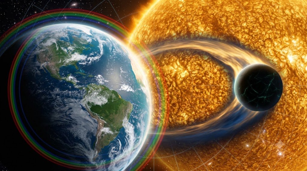
Until the final decade of the twentieth century, humanity’s knowledge of planetary systems was restricted to the single, familiar architecture of our own solar system. For centuries, philosophers and astronomers debated whether planetary systems were ubiquitous cosmic structures or miraculous flukes of astronomical history. In 1995, Michel Mayor and Didier Queloz shattered that historical isolation with the discovery of 51 Pegasi b—a scorching gas giant orbiting its host star every 4.2 days—earning them the 2019 Nobel Prize in Physics. Today, through space observatories like Kepler, TESS, and the James Webb Space Telescope (JWST), the confirmed exoplanet catalog exceeds 5,600 worlds spanning thousands of alien star systems. From blistering “Hot Jupiters” and enigmatic “Super-Earths” to temperate terrestrial worlds orbiting in the habitable zones of red dwarfs, exoplanetology has matured into one of the most vibrant and revolutionary branches of modern astrophysics. This comprehensive treatise investigates the physical detection methodologies, atmospheric characterization techniques, mass-radius degeneracies, and the empirical search for alien biosignatures.
1. Primary Exoplanet Detection Methodologies
Because planets are millions to billions of times dimmer than their host stars and separated by astronomical distances, direct imaging is extraordinarily challenging. Consequently, astronomers primarily detect exoplanets through indirect physical techniques that measure the planet’s gravitational, photometric, or astrometric influence on its host star:
The Radial Velocity (Doppler Spectroscopy) Method
A planet does not strictly orbit the center of its host star; rather, both the star and the planet orbit their common center of mass (barycenter). As the unseen planet orbits, it gravitationally tugs the host star, causing the star to wobble in a tiny counter-orbit.
When the star moves toward Earth, its spectral absorption lines are Doppler-shifted toward shorter (bluer) wavelengths; when it moves away from Earth, its lines are shifted toward longer (redder) wavelengths. The line-of-sight Radial Velocity Semi-Amplitude (K) is given by Keplerian mechanics:
K = (2πG / P)^(1/3) · (M_p · sin(i)) / (M_* + M_p)^(2/3) · (1 / √(1 – e²))
Where P is orbital period, M_p is planet mass, M_* is stellar mass, e is orbital eccentricity, and i is orbital inclination relative to the line of sight.
Because orbital inclination i is generally unknown from spectroscopy alone, radial velocity measurements yield the minimum mass of the planet: M_p · sin(i). High-precision spectrographs—such as HARPS and ESPRESSO on the Very Large Telescope—can measure stellar velocity shifts as minute as 10 centimeters per second (0.1 m/s), enabling the detection of Earth-mass worlds around nearby stars.
The Transit Photometry Method
Transit photometry occurs when an exoplanet’s orbital plane is oriented edge-on relative to Earth (i ≈ 90°), causing the planet to pass directly in front of the stellar disk during each orbit. As the opaque planetary disk transits the star, it blocks a tiny fraction of the star’s light, producing a temporary, periodic dip in the star’s photometric brightness curve.
The fractional depth of the photometric transit (ΔF / F) directly yields the ratio of the planet’s cross-sectional area to the star’s cross-sectional area:
ΔF / F = (R_p / R_* )²
For a giant planet like Jupiter transiting a Sun-like star, the dip is roughly 1% (10,000 ppm). For an Earth-sized planet transiting a Sun-like star, the dip is barely 0.0084% (84 parts per million). Detecting such subtle dips requires high-precision space telescopes positioned outside the turbulent distortion of Earth’s atmosphere, such as NASA’s Kepler and TESS missions.
| Detection Method | Physical Property Measured | Primary Observational Bias | Key Instruments & Missions |
|---|---|---|---|
| Transit Photometry | Planetary Radius (R_p), Orbital Period | Biased toward large planets in close-in orbits; requires edge-on alignment | Kepler, TESS, CoRoT, CHEOPS, PLATO |
| Radial Velocity | Minimum Mass (M_p · sin i), Eccentricity | Biased toward massive planets close to low-mass host stars | HARPS, ESPRESSO, HIRES, CARMENES |
| Direct Imaging | Thermal Luminosity, Atmospheric Spectra | Biased toward young, hot, self-luminous planets far from parent stars | SPHERE, GPI, VLT, JWST Coronagraphs |
| Gravitational Microlensing | Mass Ratio (q = M_p / M_*), Separation | Non-repeatable; sensitive to cold planets at wide orbits (~snow line) | OGLE, MOA, Nancy Grace Roman (Future) |
| Astrometry | True Mass (M_p), Full 3D Orbital Inclination | Biased toward massive planets at wide orbits around nearby stars | Gaia Space Observatory |
2. The Power of Synergy: Unlocking Bulk Density and Planetary Composition
The true gold standard of exoplanetary characterization occurs when a planet is observed by both transit photometry and radial velocity. Transit photometry delivers the physical radius R_p; radial velocity delivers the true mass M_p (because transit geometry fixes the inclination i ≈ 90°, meaning sin(i) ≈ 1).
Combining radius and mass yields the planet’s average Bulk Density (ρ_mean):
Plotting exoplanets on a Mass-Radius Diagram allows astrophysicists to determine their bulk internal composition by comparing them with theoretical equation-of-state curves: pure iron cannonballs, rocky terrestrial silicates, water-rich ocean worlds, volatile sub-Neptunes, or gas-dominated Jovian giants.
The Fulton Gap: The Evaporation Valley
Analysis of thousands of Kepler discoveries revealed a profound morphological feature known as the Fulton Gap (or Radius Valley). There is a stark deficiency of planets with radii between 1.5 and 2.0 Earth radii. Worlds bifurcate cleanly into two distinct populations: compact, rocky Super-Earths (radii < 1.5 R_Earth) and volatile-rich Sub-Neptunes with puffy hydrogen envelopes (radii 2.0–3.0 R_Earth).
Astrophysicists attribute this gap to photoevaporation and core-powered mass loss: high-energy X-ray and ultraviolet (XUV) radiation from the young host star strips away the delicate hydrogen envelopes of planets with rocky cores below a critical mass threshold, reducing them to bare, rocky Super-Earths.
Transit Timing Variations (TTV)
In multi-planetary systems, planets gravitationally interact with one another. These mutual perturbations cause the time between consecutive transits to vary slightly—a phenomenon known as Transit Timing Variations (TTV). By modeling these minute sub-minute timing shifts, astronomers can calculate the masses and orbital eccentricities of non-transiting companion planets without needing high-precision radial velocity data, an approach famously used to characterize the compact seven-planet TRAPPIST-1 system.
3. The Circumstellar Habitable Zone: Energy Balances and Boundaries
The classical Circumstellar Habitable Zone (CHZ), formalized by James Kasting and Ravi Kumar Kopparapu, defines the range of orbital distances where a rocky terrestrial planet with an Earth-like atmosphere could sustain liquid water oceans on its surface under atmospheric equilibrium:
Inner Edge: The Runaway and Moist Greenhouse Limits
The inner boundary of the habitable zone is set by the Runaway Greenhouse Limit (roughly 0.95 AU for a solar twin). Closer in, surface temperatures cause ocean water to evaporate into the stratosphere, where stellar UV photolysis dissociates water into hydrogen and oxygen, leading to irreversible hydrodynamic water loss into space (the Venusian fate).
Outer Edge: The Maximum Greenhouse Limit
The outer boundary is set by the Maximum Greenhouse Limit (roughly 1.67 AU for a solar twin). Beyond this orbit, even a thick atmosphere of 100% carbon dioxide cannot keep surface temperatures above freezing because Rayleigh scattering from the dense gas reflects more incoming sunlight than the greenhouse effect traps, causing atmospheric collapse and global glaciation (the Martian fate).
Because M-dwarf stars (red dwarfs) are much cooler and dimmer than the Sun (luminosities of 0.001 to 0.01 L☉), their habitable zones sit exceptionally close in—often between 0.05 and 0.2 AU (orbital periods of days or weeks). The famous TRAPPIST-1 system packs seven Earth-sized worlds within an orbital radius smaller than Mercury’s orbit around the Sun, with three planets (TRAPPIST-1e, 1f, and 1g) orbiting within the habitable zone. However, planets orbiting in M-dwarf habitable zones face severe challenges: they are almost certainly tidally locked (one face permanently roasted by the star, the other frozen in eternal darkness) and subject to ferocious stellar flares and coronal mass ejections that can strip planetary atmospheres away entirely.
4. Atmospheric Characterization: Transmission and Emission Spectroscopy
Finding a planet in the habitable zone is merely the first step; confirming habitability requires probing its atmosphere. The premier technique for this is Transmission Spectroscopy, deployed with revolutionary precision by the James Webb Space Telescope (JWST).
During a transit, while the opaque solid core of the planet blocks starlight directly, a thin annulus of starlight filters through the transparent upper layers of the planet’s atmosphere. Atoms and molecules in the atmosphere absorb specific discrete wavelengths of starlight:
- At wavelengths where atmospheric molecules absorb light (e.g., water vapor at 1.4 μm and 1.9 μm; carbon dioxide at 4.3 μm; methane at 3.3 μm), the atmosphere appears opaque, making the planet look slightly larger and producing a deeper transit depth.
- At transparent wavelengths, starlight passes unhindered, making the transit dip slightly shallower.
By measuring the transit depth across thousands of infrared wavelengths, JWST constructs an atmospheric transmission spectrum. JWST has already made landmark discoveries, confirming atmospheric carbon dioxide on WASP-39b, sulfur dioxide photochemical hazes, water vapor absorption, and measuring the thermal emission of TRAPPIST-1b.
The Rossiter-McLaughlin Effect and Spin-Orbit Alignment
As a star rotates, one hemisphere rotates toward the observer (blueshifted) while the other rotates away (redshifted). When a transiting planet passes across the blueshifted stellar hemisphere, it blocks blue light, causing the apparent integrated light of the star to appear redshifted. As the planet crosses to the redshifted hemisphere, the light appears blueshifted. This spectroscopic anomaly—the Rossiter-McLaughlin Effect—enables astronomers to measure the true stellar obliquity (the angle between the stellar spin axis and the planetary orbital plane). Many Hot Jupiters exhibit wildly misaligned, polar, or even retrograde orbits, proving that violent gravitational scatterings and Kozai-Lidov disk migrations reshuffled these planetary systems early in their lifespans.
5. The Search for Atmospheric Biosignatures and Technosignatures
What specific molecular combinations would prove that an exoplanet harbors biological life? Astrobiologists focus on Atmospheric Biosignatures—gaseous chemical species produced by biological metabolisms that exist in extreme thermodynamic disequilibrium with their chemical environment:
1. Oxygen (O₂) and Ozone (O₃): Oxygen is hyper-reactive; without continuous replenishment by oxygenic photosynthesis (such as plants and cyanobacteria on Earth), atmospheric oxygen would rapidly react with surface minerals and vanish within geological moments.
2. Methane (CH₄) in the presence of Oxygen: Methane reacts rapidly with oxygen in the presence of sunlight to form carbon dioxide and water. The simultaneous detection of abundant methane alongside oxygen or ozone in an exoplanetary atmosphere is the classic “smoking gun” biosignature, because no known abiotic geochemical process can maintain both species simultaneously in high quantities.
3. Nitrous Oxide (N₂O): “Laughing gas” on Earth is produced almost exclusively by microbial nitrogen-fixing bacteria through denitrification pathways.
False Positives and Abiotic Mimics
Astrobiologists exercise rigorous skepticism regarding “false positives.” For example, extreme ultraviolet photolysis of water vapor in an ocean-desiccating atmosphere can produce abiotic oxygen without life. To confirm a true biological origin, astronomers must comprehensively model the host star’s UV spectrum, atmospheric humidity, and the absence of abiotic indicator gases like carbon monoxide (CO), which biological ecosystems on Earth actively metabolize.
6. The Future of Exoplanet Exploration: The Habitable Worlds Observatory
The coming decades will witness the deployment of next-generation observatories engineered specifically to image and characterize Earth-like twins orbiting sun-like stars. Ground-based Extremely Large Telescopes (the 39-meter ELT and the Thirty Meter Telescope) will utilize advanced adaptive optics to directly resolve exoplanets from ground level.
In space, NASA’s prioritized flagship mission for the 2030s—the Habitable Worlds Observatory (HWO)—will employ a 6-meter optical/UV space telescope equipped with an ultra-precise coronagraph capable of suppressing host starlight by a factor of 10 billion to 1. The HWO is designed with the express scientific mandate to directly image and spectroscopically analyze at least 25 habitable terrestrial worlds, searching for the telltale signatures of oxygen, ozone, water vapor, and chlorophyll-like surface vegetation reflection (“the Red Edge”). We stand upon the threshold of an epochal discovery: the moment when humanity looks up at a distant star and knows, with empirical physical certainty, that we are not alone.